3.6.2 Math Editor Examples

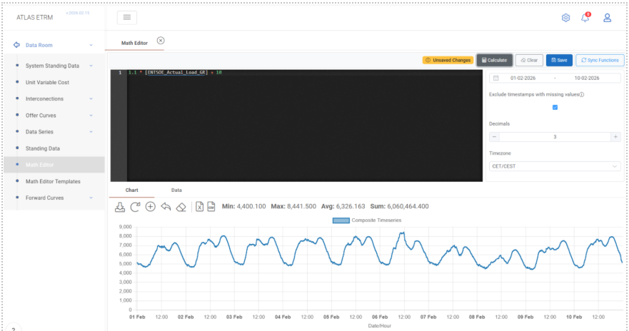
Example 01 – MULTIPLICATION / SUMMATION 

Expression 

1.1 * [ENTSOE_Actual_Load_GR] + 10 

This example creates a calculated time series based on an existing data series (ENTSOE_Actual_Load_GR). The formula increases the original 15-minute system load by 10% and then adds a constant value of 10 MW. The result is a modified load profile derived directly from the underlying series. 

Data series are referenced inside square brackets [ ]. When the user starts typing the name of a series, the system provides autocomplete suggestions from the Data Room, so the full name does not need to be typed manually. The wildcard character * can be used during search to combine keywords and locate a series more efficiently.  

Standard arithmetic operators such as +, -, *, and / are supported directly within the expression editor. 

To execute the calculation, the user selects the desired date range, defines the number of decimals, optionally enables “Exclude timestamps with missing values”, and clicks Calculate. The result is displayed below in both chart and data format. If required, the calculated series can then be stored using Save. 

Such transformations are typically used to apply adjustment factors, create alternative load scenarios, or generate modified profiles that can later be reused in further calculations, dashboards, or deal-related configurations. 

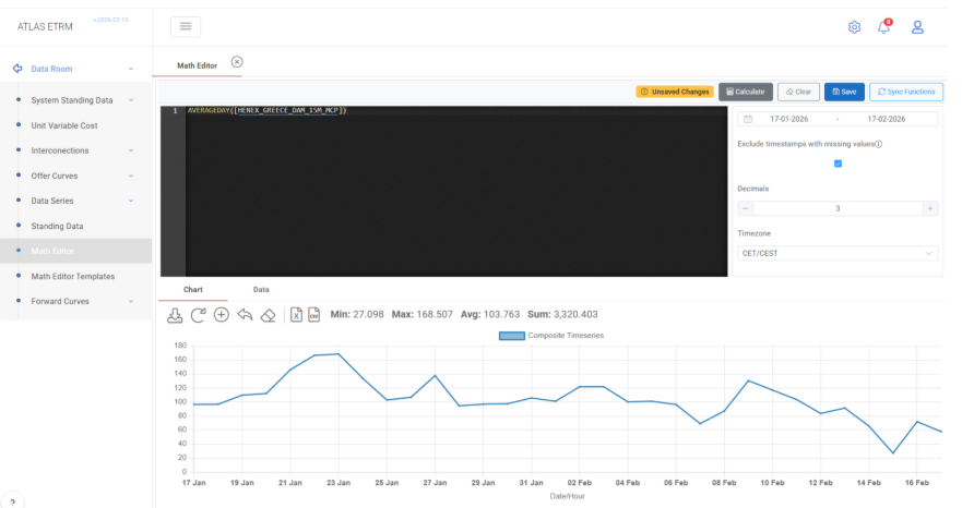
Example 02 – AVERAGEDAY 

Expression 

AVERAGEDAY([HENEX_GREECE_DAM_15M_MCP]) 

This example generates a new data series from the 15-minute market price series HENEX_GREECE_DAM_15M_MCP. The function AVERAGEDAY() converts a higher-frequency time series (e.g. 15-minute data) into daily granularity by calculating, for each calendar day, the arithmetic mean of all underlying values. Each resulting daily value therefore represents the average DAM price of that specific day.

The input series is referenced inside square brackets [ ], while the function name is written followed by parentheses containing the argument. The function accepts a single time series as input and performs a temporal aggregation without altering the underlying price logic—only its granularity. 

This type of calculation is useful whenever higher-frequency data needs to be aligned with daily-level analysis. By converting hourly or sub-hourly values into daily averages, the user can simplify volatility, standardize reporting intervals, and prepare data for use in KPIs, structured calculations, portfolio summaries, or other analytical processes that operate daily. 

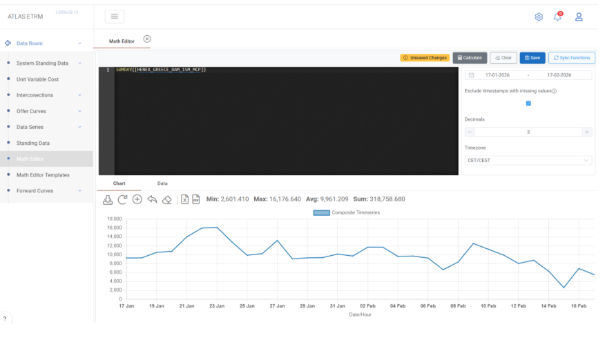
Example 03 – SUMDAY

Expression

SUMDAY([HENEXGREECEDAM15MMCP])

This example generates a new daily data series from the 15-minute market price series HENEXGREECEDAM15MMCP. The function SUMDAY() performs temporal aggregation by summing all underlying values within each calendar day and assigning the total to the respective day. The resulting series therefore has daily granularity, where each value represents the sum of all quarter-hour MCP values for that specific date.

The input data series is referenced inside square brackets [ ]. The SUMDAY() function accepts a higher-frequency time series (e.g., 15-minute) and applies downsampling to Day granularity using summation as the aggregation method. The output preserves the numeric type of the original series while modifying its time resolution.

Optionally, SUMDAY() supports a second boolean parameter (ignoreNulls). When set to true, null values within the aggregation range are ignored. When set to false (default behavior), the presence of any null value within the day results in a null output for that day. This provides control over how incomplete datasets are treated during aggregation. The ignoreNulls optional parameter is available for all downsampling functions such as SUM, AVERAGE and DOWNSAMPLE.

Such aggregation logic is typically used when transforming high-frequency volume or quantity data into daily totals, preparing inputs for settlement calculations, aligning datasets to daily KPIs, or constructing summarized reports where daily-level analysis is required.

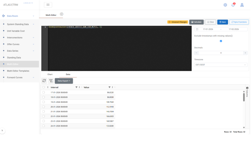
Example 04 – ROUND 

Expression 
ROUND(AVERAGEDAY([HENEX_GREECE_DAM_15M_MCP]), 4) 

 This example creates a calculated data series by first converting the 15-minute DAM price series HENEX_GREECE_DAM_15M_MCP into daily granularity using the AVERAGEDAY() function and then rounding each resulting daily value to four decimal places using the ROUND() function. 

The expression demonstrates nested function usage. The inner function AVERAGEDAY() performs temporal aggregation and returns a daily series where each value represents the arithmetic mean of the hourly prices for the respective day. The outer function ROUND() then adjusts the numeric precision of each daily value without modifying its granularity or underlying price logic. 

The ROUND() function accepts either a time series, standing data field, or scalar as input. When a second parameter is provided, it specifies the number of decimal places to be retained. If the decimal parameter is omitted, rounding is performed to the nearest integer by default. 

This type of transformation is typically applied when standardizing numerical precision for reporting, settlement calculations, KPI construction, or export processes where fixed decimal formatting is required. It ensures consistency in downstream analytics while preserving the economic meaning of the original data. 

Example 05 – COLLAR/CAP/FLOOR 

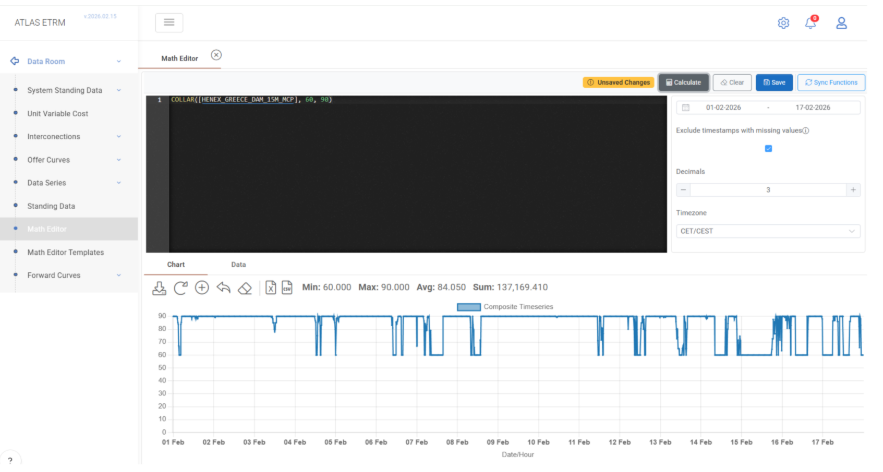
Expression 
COLLAR([HENEX_GREECE_DAM_15M_MCP], 60, 90) 

This example creates a constrained version of the 15-minute DAM price series HENEX_GREECE_DAM_15M_MCP by applying lower and upper bounds to each timestamp value. The COLLAR() function enforces a floor of 60 and a cap of 90 on the original series. 

For each quarter-hour value: 
– If the price is below 60, it is raised to 60. 
– If the price is above 90, it is reduced to 90. 
– If the price lies between 60 and 90, it remains unchanged. 

The input time series is referenced inside square brackets [ ]. The second parameter defines the FloorValue, while the third parameter defines the CapValue. Both can be scalar constants, standing numeric fields, or time-dependent standing series, allowing either fixed or dynamic boundaries per timestamp. 

The COLLAR() function does not alter the granularity or time structure of the original series; it only adjusts numeric values that fall outside the specified interval. The resulting data series preserves the original frequency while ensuring that all values remain within the defined price band. 

Such bounded transformations are commonly used in risk management, contract modelling, structured products, and scenario analysis. They are particularly useful when simulating price caps, regulatory thresholds, or risk-controlled exposure profiles where extreme values must be limited within predefined ranges.

Example 06 – ABS 

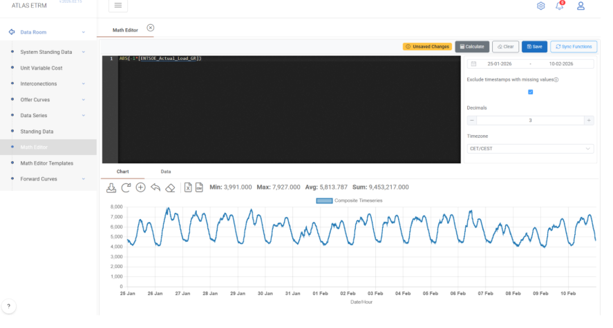
Expression 
ABS(-1 * [ENTSOE_Actual_Load_GR]) 

This example generates a new time series by first multiplying the 15-minute system load series ENTSOE_Actual_Load_GR by -1 and then applying the ABS() function to the result. 

The multiplication by -1 reverses the sign of each timestamp value, transforming positive load values into negative ones. The ABS() function then converts each value to its absolute magnitude, effectively removing the sign and returning only non-negative values. The final output therefore mirrors the original load series in magnitude, regardless of intermediate sign changes. 

The input time series is referenced inside square brackets [ ], while ABS() accepts either a time series, a standing numeric field, or a scalar numeric value. When applied to a time series, the function operates per timestamp, preserving the original granularity and time structure while modifying only the numeric sign. 

This type of transformation is commonly used in analytical scenarios where direction (positive/negative sign) is irrelevant and only magnitude is required. Typical use cases include deviation analysis, imbalance calculations, absolute error metrics (e.g., components of MAPE), or normalization steps in more complex mathematical expressions. 

Example 07 – POWER 

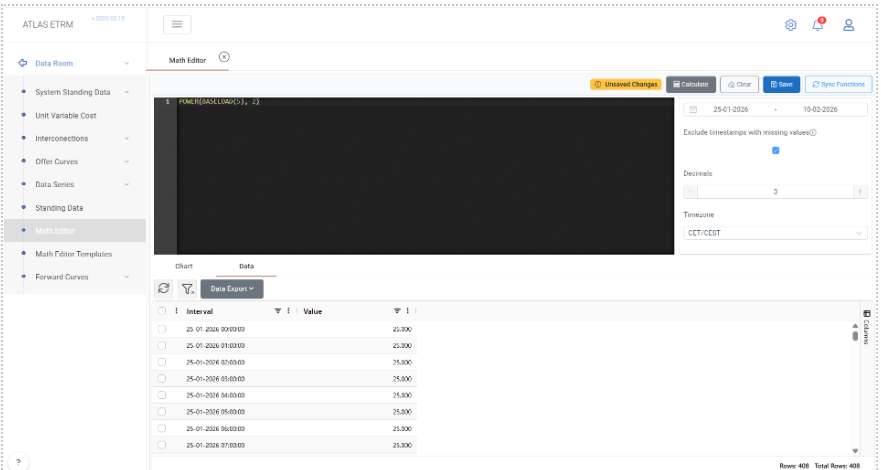
Expression 
POWER(BASELOAD(5), 2) 

 This example creates a calculated time series by first generating a synthetic hourly baseload profile using BASELOAD(5) and then raising each value of that series to the power of 2 using the POWER() function. 

The BASELOAD(5) function produces an hourly time series where each timestamp has a constant value of 5. The POWER() function then applies an exponential transformation, calculating 5² for each hourly value. As a result, the produced series contains the value 25 for every hour in the selected date range. 

The POWER() function accepts as its first argument a time series, standing data field, or scalar value. The second argument defines the exponent and may be either a scalar numeric value or a standing numeric field. When applied to a time series, the operation is performed per timestamp, preserving the original granularity and time structure. 

Exponential transformations are commonly used in advanced analytical modelling, nonlinear scenario construction, sensitivity analysis, and mathematical simulations where squared or higher-order effects must be incorporated into pricing, volume modelling, or KPI calculations. 

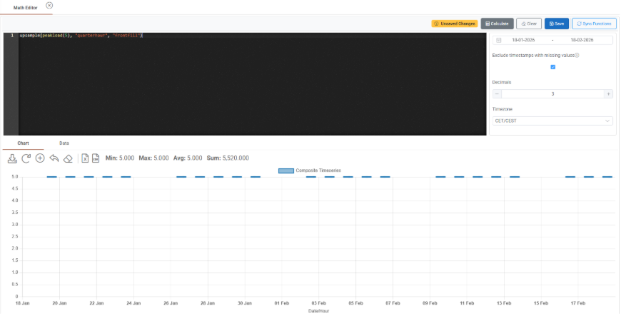
Functions BASELOAD, PEAKLOAD, OFFPEAKLOAD produce an hourly output. In case the user wants to produce a load profile in a higher granularity, the upsample function can be used, e.g. upsample (peakload(5), "quarterhour", "frontfill") produces a peakload of 5 with a quarterly granularity:

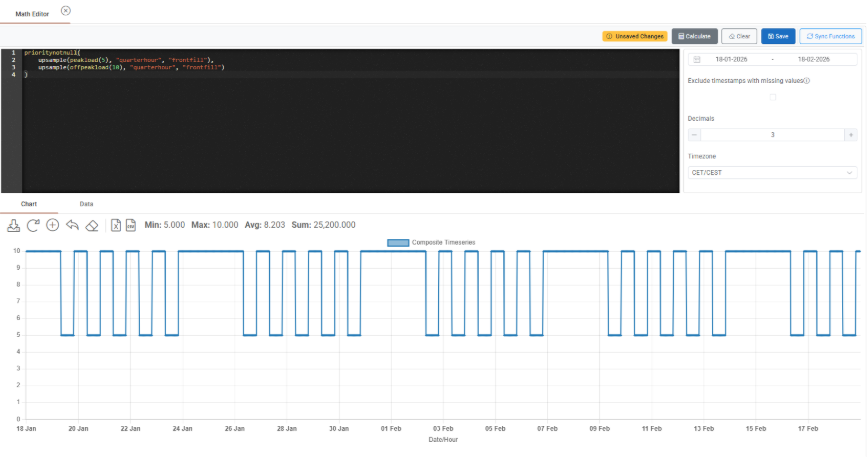
Of course the user can combine multiple profiles, e.g. a peakload and an offpeakload using a combination of these functions and the prioritynotnull function:

Example 08 – SHIFTMONTH 

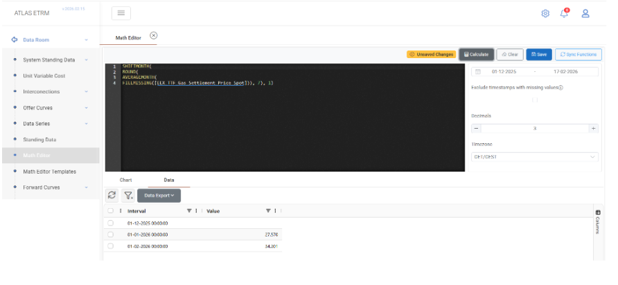
Expression 
SHIFTMONTH( 
ROUND( 
AVERAGEMONTH( 
FILLMISSING([EEX_TTF_Gas_Settlement_Price_Spot])), 7), 1) 

This example demonstrates a multi-step transformation pipeline applied to the EEX_TTF_Gas_Settlement_Price_Spot time series, combining data cleansing, temporal aggregation, precision control, and calendar shifting. 

The calculation is executed in the following logical sequence: 

1. FILLMISSING() fills any gaps in the original time series. If missing timestamps exist, they are forward-filled using the last available non-null value. This ensures continuity of the dataset before aggregation. 

2. AVERAGEMONTH() converts the gas settlement prices into monthly granularity by calculating the arithmetic mean of all values within each calendar month. The result is a monthly average price series. 

3. ROUND(…, 7) standardizes the numeric precision of the monthly averages to seven decimal places. This step does not alter the granularity, only the formatting and stored precision. 

4. SHIFTMONTH(…, 1) shifts the resulting monthly series by one month forward. The time keys remain unchanged, but each timestamp now contains the value from one month earlier (t - 1 month). A positive shift value creates a lagged series, while a negative value would produce a lead (future) shift. 

The final output is therefore a lagged monthly average gas price series with standardized precision and no missing values. 

Such chained transformations are common in commodity market analysis, especially when constructing index-linked pricing formulas, settlement references (e.g., previous month average), rolling benchmarks, or backward-looking KPIs used in contract pricing mechanisms. 

Example 09 – DAYSOFMONTH 

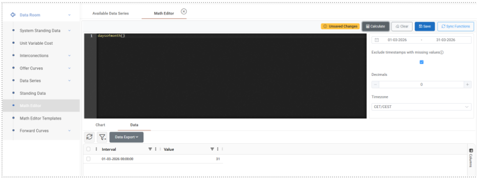
Expression 
DAYSOFMONTH() 

This example generates a synthetic monthly time series where each timestamp represents a calendar month and its value corresponds to the total number of days contained in that specific month. 

The DAYSOFMONTH() function does not require any input time series. Instead, it creates a new series dynamically based on the selected date range in the Math Editor. For each month included in the calculation window, the function determines whether the month has 28, 29, 30, or 31 days and assigns that number as the monthly value. Leap years are automatically handled by the system, meaning that February will contain 29 days when applicable. 

The resulting series has monthly granularity and numeric values. The time keys correspond to calendar months, while the data values represent the number of calendar days in each respective month. 

This function is commonly used in settlement calculations, normalization processes, weighted averages, prorating logic, and volumetric conversions where the number of days per month is required as a multiplier or divisor in structured pricing formulas or KPI computations. 

Example 10 – MAX 

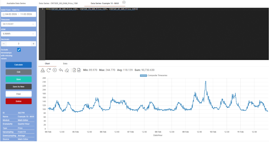
Expression 
MAX([ENTSOE_GR_DAM_Price_15M], [ENTSOE_FR_DAM_Price_15M], [ENTSOE_DE_DAM_Price_15M]) 

This example creates a new calculated time series that, for each timestamp, returns the maximum value among three hourly DAM price series: ENTSOE_GR_DAM_Price_15M, ENTSOE_FR_DAM_Price_15M, and ENTSOE_DE_DAM_Price_15M. 

The MAX() function operates per timestamp when multiple time series are provided. For every time-step in the selected date range, the function compares the corresponding price values of the three markets and selects the highest one. The resulting series preserves the original granularity  and contains, at each time step, the maximum price observed among the specified bidding zones. 

All input time series are referenced inside square brackets [ ]. The function can accept one or more time series, as well as numeric standing fields or scalar values. When scalar values are included, they act as minimum thresholds. In contrast, when multiple time series are provided—as in this example—the function performs a direct cross-series comparison per timestamp. 

Such calculations are typically used in cross-border market analysis, price coupling evaluation, congestion studies, and structured pricing mechanisms where exposure depends on the highest observed price among a group of markets. This type of logic is also relevant for cap/floor clauses, optimization strategies, and comparative benchmarking across bidding zones. 

Example 11 – MAXMONTH 

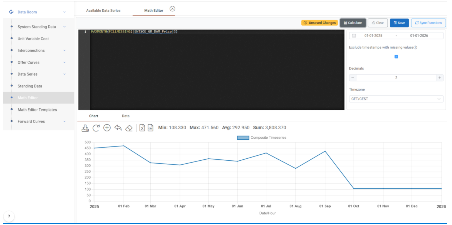
Expression 
MAXMONTH(FILLMISSING([HENEX_GREECE_DAM_15M_MCP])) 

This example creates a monthly data series derived from the 15-minute DAM price series HENEX_GREECE_DAM_15M_MCP. The calculation combines data cleansing and temporal downsampling in order to obtain, for each calendar month, the maximum observed hourly price. 

The execution logic is sequential: 

1. FILLMISSING() is first applied to the original time series. Any missing values are forward-filled using the last available non-null observation. This ensures that potential data gaps do not propagate null results during the aggregation stage. 

2. MAXMONTH() then performs downsampling to Month granularity. For each calendar month within the selected date range, the function identifies the highest hourly value and assigns that value to the corresponding monthly timestamp. 

The resulting series has monthly frequency and numeric values. Each monthly data point represents the peak DAM price recorded during that month. The time structure is adjusted to monthly keys, while the aggregation logic strictly applies a maximum operator over the underlying higher-frequency data. 

This type of calculation is typically used in peak exposure assessment, structured contract clauses linked to monthly maximum prices, stress testing scenarios, and market volatility analysis where the highest intra-month price is economically relevant. 

Example 12 - MINMONTH

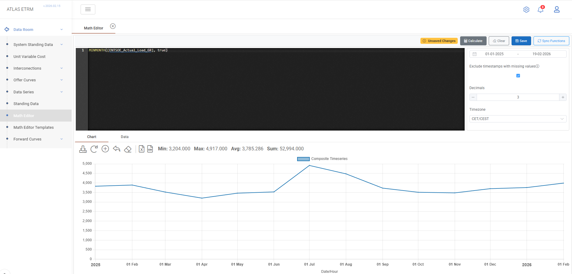
Expression
MINMONTH([ENTSOE_Actual_Load_GR], true)

This example generates a monthly time series representing the minimum observed system load for each calendar month, based on a 15-minute (QuarterHour) load series.

The MINMONTH() function performs downsampling from QuarterHour granularity to Month granularity. For each calendar month, it evaluates all underlying 15-minute load values and selects the lowest one recorded during that month.

The second parameter (true) activates the ignoreNulls behaviour. When enabled, null values within the aggregation window are excluded from the calculation. If it were set to false (default), the presence of null values within a month could result in a null output for that entire month.

The resulting output is a SimpleDataNumeric time series with Month granularity. Each monthly timestamp represents the minimum 15-minute load observed within the respective month.

Such calculations are typically used in demand floor analysis, system adequacy monitoring, infrastructure base-load assessment, and seasonal benchmarking where the lowest intra-month load level is analytically relevant.

Example 13 – PRIORITYNOTNULL 

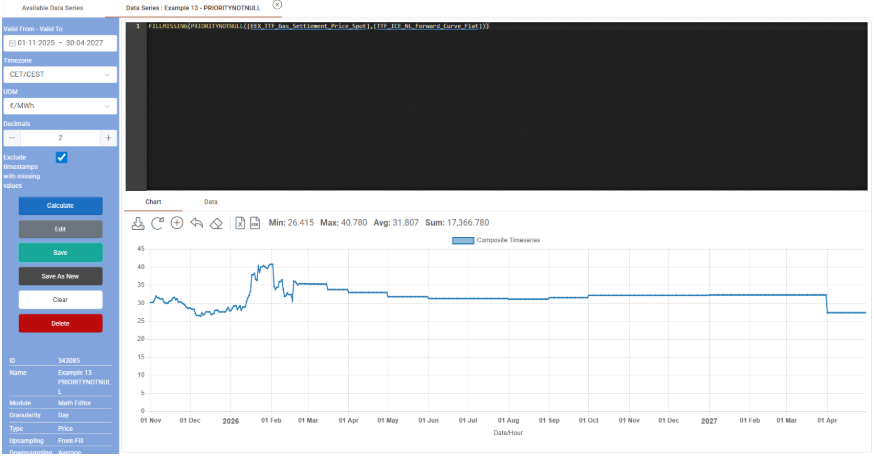
Expression 
FILLMISSING(PRIORITYNOTNULL([EEX_TTF_Gas_Settlement_Price_Spot],[TTF_ICE_NL_Forward_Curve_Flat]))  

This example demonstrates the combination of fallback selection logic and gap-filling in order to construct a continuous gas price time series. 

The calculation is evaluated in two stages: 

1. PRIORITYNOTNULL() operates per timestamp and evaluates its arguments in the order provided. For each time step: 
   – If the first time series contains a non-null value, that value is returned. 
   – If the first time series is null, the function evaluates the second time series and returns its value instead. 
   – If all provided arguments are null at a given timestamp, the result remains null. 

   Note: PRIORITYNOTNULL accepts 2 or more inputs, so this logic is also valid for the 3rd, 4th etc. Timeseries. 

   This structure enables the implementation of fallback pricing logic, where a secondary data source is automatically used when the primary one is unavailable. The operation is performed per timestamp and preserves the original granularity of the series. 

2. FILLMISSING() is then applied to the resulting series. Any remaining missing timestamps are forward-filled using the last available non-null observation. The final output is a cleaned and continuous time series with the same frequency as the input data. It incorporates hierarchical source selection and systematic null handling. 

Such logic is typically used in index construction, MTM (Mark-to-Market) calculations, contract pricing mechanisms with backup references, and analytical workflows where uninterrupted time series are required for settlement, valuation, or KPI computations.

Example 14 – TODATE 

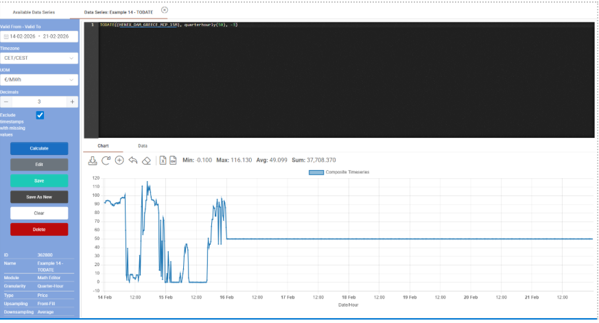
Expression 
TODATE([HENEX_DAM_GREECE_MCP_15M], QUARTERHOURLY(50), -3) 

This example combines two time series of the same granularity into a single spliced series, using a date-based switching rule relative to today. 

The TODATE() function operates as follows: 

• The first argument, HENEX_DAM_GREECE_MCP_15M, is used up to (today + DaysValue). 

• The second argument, QUARTERHOURLY(50), is used from (today + DaysValue + 1) onward. 

In this case, DaysValue is -3. Therefore: 

• The DAM price series is used up to three days before today. 

• From two days before today onward, the value is replaced by  QUARTERHOURLY (50), which produces a constant quarter-hourly series with value 50. 

The comparison is performed in local wall-time for sub-day series, meaning that quarter-hour timestamps are evaluated according to calendar logic rather than pure index position. The resulting series preserves the original frequency (QuarterHour) and maintains a continuous time structure. 

This type of splicing logic is commonly used when combining realized and forecast data. Typical applications include: 

• Using historical actual prices up to a cut-off date and forecast values thereafter. 

• Implementing rolling valuation curves. 

• Constructing hybrid series that transition from observed market data to modelled assumptions. 

The TODATE() function therefore enables dynamic switching between datasets based on relative calendar logic, supporting flexible analytical and contract modelling workflows. 

Example 15 – GRANULAR_PRICE 

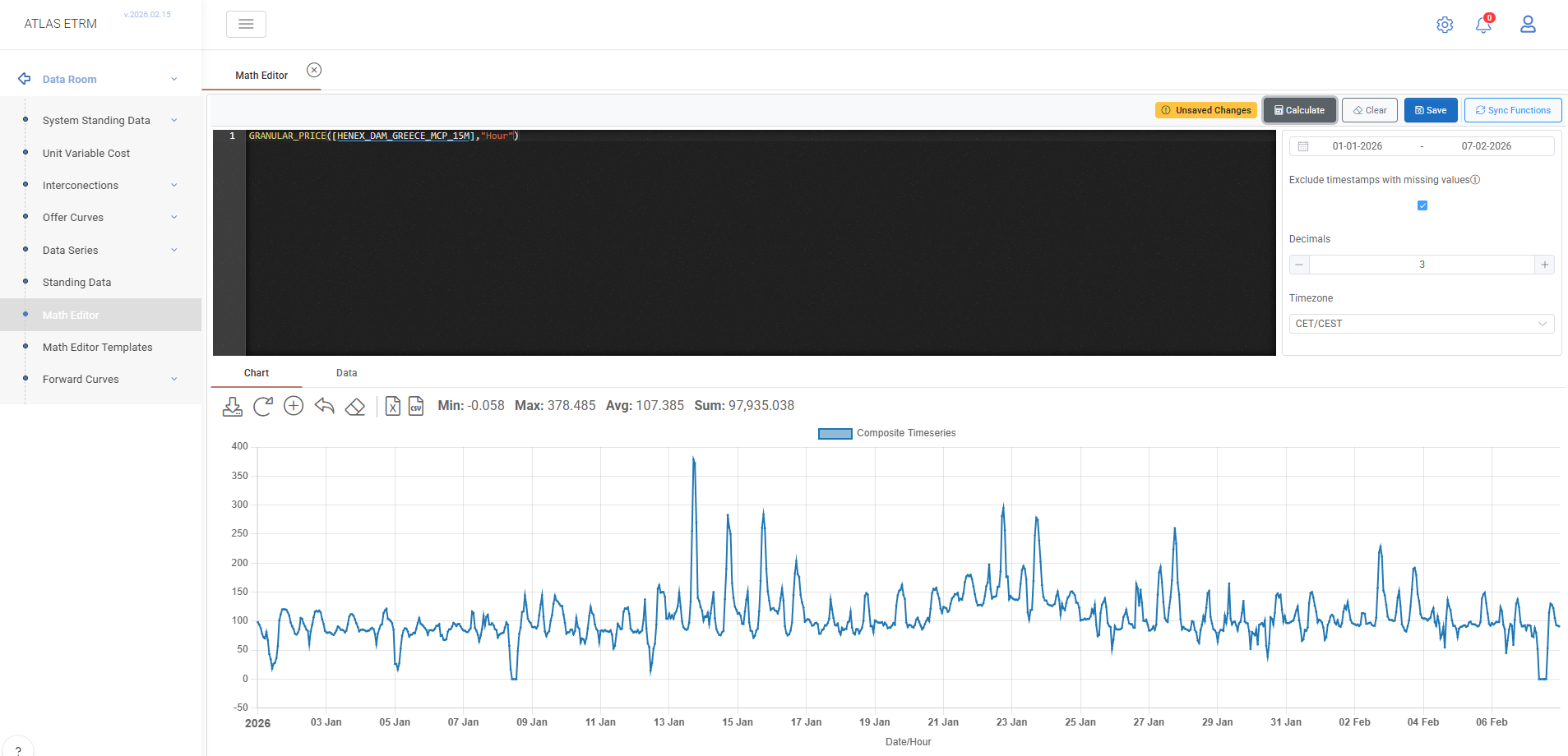
Expression 
GRANULAR_PRICE([HENEX_DAM_GREECE_MCP_15M], "Hour") 

This example resamples the price time series HENEX_DAM_GREECE_MCP_15M from QuarterHour granularity to Hour granularity. The function GRANULAR_PRICE() adjusts the temporal resolution of a price series while preserving its economic interpretation. 

Because the original series has a finer granularity (15-minute), the function performs downsampling. In this case, all quarter-hour values within each calendar hour are aggregated, and their arithmetic average defines the value of that hour. For price series specifically, downsampling always applies averaging logic rather than summation. 

If the operation were performed in the opposite direction (e.g., from hourly to quarter-hourly), upsampling would replicate the hourly value across all sub-intervals within that hour. 

The resulting series is a SimpleDataNumeric time series with Hour granularity. The time structure is aligned to hourly timestamps, and each hourly value represents the average of the four underlying 15-minute price observations. 

An optional third parameter (ignoreNulls) may be used to define null-handling behaviour during downsampling. When set to true, null values are skipped; when false (default), the presence of null values may produce a null result for the aggregated period. 

Such granularity transformations are frequently required in settlement alignment, cross-market comparisons, portfolio simulations, and contract modelling where datasets must be standardized to a common temporal resolution. 

Example 16 – IFDATE 

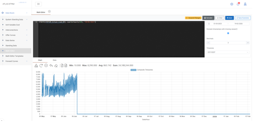
Expression 
IFDATE([ENTSOE_Actual_Load_GR],  QUARTERHOURLY(10), "20/06/2025") 

 This example creates a hybrid time series by switching between two data sources based on a fixed calendar date. 

The IFDATE() function evaluates each timestamp using local wall-time comparison logic. For every time step: 

• If the timestamp is before 20/06/2025, the value is taken from  ENTSOE_Actual_Load_GR . 

• If the timestamp is on or after 20/06/2025, the value is taken from QUARTERHOURLY(10), which produces a constant hourly series with value 10. 

The left-hand side (LHS) argument must be a time series. The right-hand side (RHS) argument can be either a time series or a scalar. In this case,  QUARTERHOURLY (10) generates a time series that matches the frequency of the original load series. 

The resulting series preserves the original granularity  and applies a deterministic structural break at the specified date. Unlike TODATE(), which switches relative to today, IFDATE() uses a fixed calendar date explicitly defined in the expression. 

Such date-based switching logic is typically used in scenario modelling, regulatory changes, contract amendments, forecast transitions, or structural adjustments where different pricing or volume logic must apply from a specific effective date onward. 

Example 17 – IFDATEVALUE 

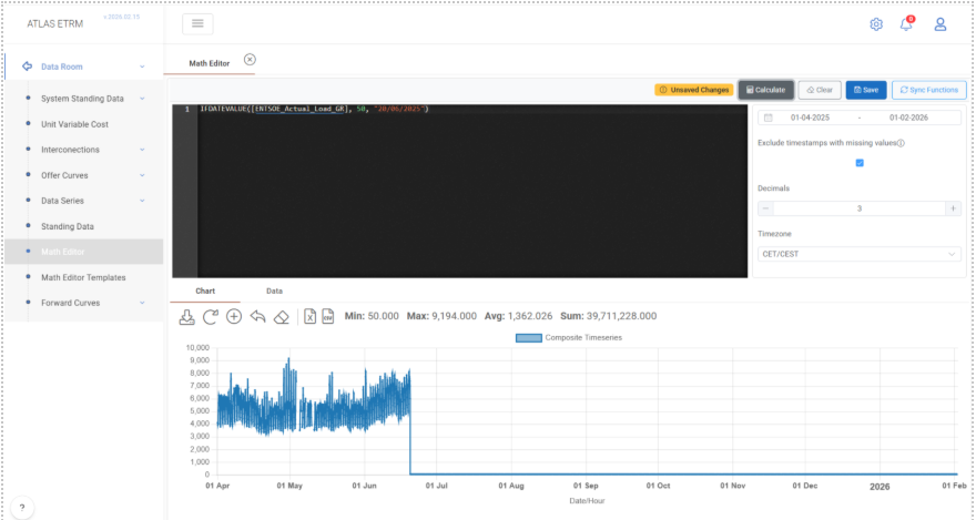
Expression 
IFDATEVALUE([ENTSOE_Actual_Load_GR], 50, "20/06/2025") 

This example creates a modified load time series by applying a date-based override using a fixed scalar value. 

The IFDATEVALUE() function evaluates each timestamp using local wall-time comparison logic. For every time step: 

• If the timestamp is before 20/06/2025, the value is taken from ENTSOE_Actual_Load_GR. 

• If the timestamp is on or after 20/06/2025, the value is replaced by the scalar value 50. 

Unlike IFDATE(), where both arguments may be time series, IFDATEVALUE() explicitly replaces the original data with a numeric constant after the specified date. The original granularity of the time series (e.g., hourly) is preserved, and the scalar value is applied uniformly to all timestamps from the effective date onward. 

The resulting series therefore contains historical actual load values up to the defined date and a constant projected value thereafter. 

Such logic is typically used in scenario simulations, stress testing, regulatory cap implementations, or simplified forward assumptions where a constant parameter must apply from a specific effective date while retaining historical data unchanged. 

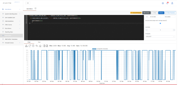
Example 18 – IF 

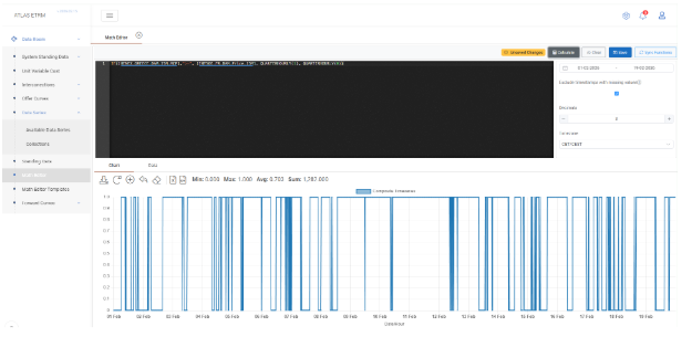
Expression 

IF([HENEX_GREECE_DAM_15M_MCP],">=", [ENTSOE_FR_DAM_Price_15M], QUARTERHOURLY(1), QUARTERHOURLY(0)) 

This example creates a conditional quarter-hourly time series based on the comparison between two market price series:  HENEX_GREECE_DAM_15M_MCP and  ENTSOE_FR_DAM_Price_15M. 

The IF() function evaluates the condition per timestamp using the specified comparison operator. In this case: 

• For each hour, if the Greek DAM price is greater than or equal to the French DAM price, the function returns QUARTERHOURLY(1). 

• Otherwise, it returns QUARTERHOURLY(0). 

The operator ">=" performs a per-timestamp numeric comparison between the two input time series. The result of the condition determines which value is selected for that specific hour. 

QUARTERHOURLY(1) and QUARTERHOURLY(0) generate constant 15-minute time series with values 1 and 0 respectively. Because the condition itself is evaluated quarter-hourly, the output preserves the same granularity. The final result is therefore a binary indicator series (1/0) showing whether the Greek DAM price is higher than or equal to the French DAM price at each time step. 

Such conditional logic is frequently used in spread analysis, market dominance indicators, cross-border price comparisons, trigger-based settlement clauses, and algorithmic signal generation. It enables the creation of rule-based datasets that can subsequently be aggregated, analysed, or integrated into more complex pricing and risk calculations. 

Example 19 – NESTED IF 

Expression 
IF([ HENEX_GREECE_DAM_15M_MCP], "<", [, ENTSOE_FR_DAM_Price_15M], QUARTERHOURLY(0),  

   IF([ HENEX_GREECE_DAM_15M_MCP], "==", [ ENTSOE_FR_DAM_Price_15M], QUARTERHOURLY(10),      

      QUARTERHOURLY(15))) 

This example demonstrates the use of nested conditional logic in order to evaluate multiple comparison outcomes between two hourly market price series. 

The outer IF() function first evaluates whether the Greek DAM price is strictly lower than the French DAM price for each timestamp: 

• If the condition is true, the result is QUARTERHOURLY(0). 

• If the condition is false, the evaluation proceeds to the inner IF() statement. 

The inner IF() then checks whether the two prices are equal: 

• If the prices are equal, the function returns QUARTERHOURLY(10). 

• If neither condition (lower nor equal) is satisfied, it implies that the Greek DAM price is greater than the French DAM price, and the function returns QUARTERHOURLY(15). 

Because QUARTERHOURLY() generates constant 15-minute time series, the final result preserves quarter-hourly granularity and produces a categorical indicator series with three possible values: 
0 → Greek price lower than French 
10 → Prices equal 
15 → Greek price higher than French 

Nested IF structures allow multi-branch logical evaluation and are commonly used in spread-based classification, rule-based pricing mechanisms, tariff logic, threshold modelling, and algorithmic decision frameworks where more than two conditional outcomes must be represented. 

Example 20 – BAND / BUSINESSDAYS 

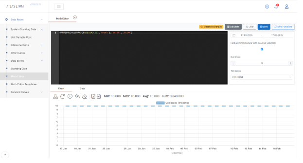
Expression 
BAND(BUSINESSDAYS(BASELOAD(10), "Greek"), "08:00", "20:00") 

This example constructs a calendar- and time-filtered hourly time series by combining BUSINESSDAYS() and BAND(). 

The execution flow is as follows: 

1. BASELOAD(10) generates a constant hourly time series with value 10 for all timestamps within the selected date range. 

2. BUSINESSDAYS(BASELOAD(10), "Greek") applies Greek calendar logic to the hourly series. Only timestamps that correspond to Greek business days (excluding weekends and official holidays defined in the calendar) retain their values. Non-business days are excluded according to the calendar rules. The resulting series preserves hourly granularity. 

3. BAND(…, "08:00", "20:00") further filters the series by restricting values to the specified intra-day time window. For each valid business day, only the hours between 08:00 and 20:00 are retained. Timestamps outside this band are excluded. 

The final output is therefore an hourly time series with value 10, valid only during Greek business days and only within the defined time-of-day interval. 

Such combined calendar and time-band filtering is typically used for peak-hour product construction, working-hours exposure modelling, tariff window simulation, delivery block definition, and structured contracts where both calendar eligibility and intra-day constraints must be enforced simultaneously. 

Example 21 – PEAKLOAD 

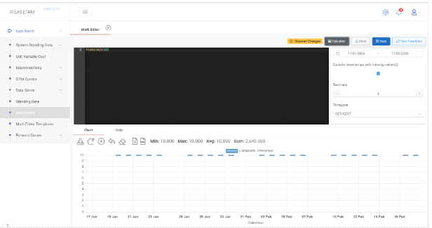
Expression 
PEAKLOAD(10) 

This example generates an hourly peak-load time series with a constant value of 10 during predefined peak hours. 

The PEAKLOAD() function creates a synthetic hourly series where: 

• For Monday to Friday, between 08:00 and 20:00, the value is set to 10. 

• For all other hours (including nights and weekends), the value is 0. 

The resulting time series has Hour granularity and automatically applies the standard peak-hour definition (weekday business hours). No input time series is required, as the function internally constructs the profile based on calendar and time-of-day rules. 

The output is a SimpleDataNumeric series that represents a structured delivery block commonly used in electricity markets. 

Such peak-load profiles are typically applied in power trading, contract modelling, structured products, and settlement simulations where delivery is limited to predefined peak hours rather than continuous baseload supply. 

Example 22 – OFFPEAKLOAD 

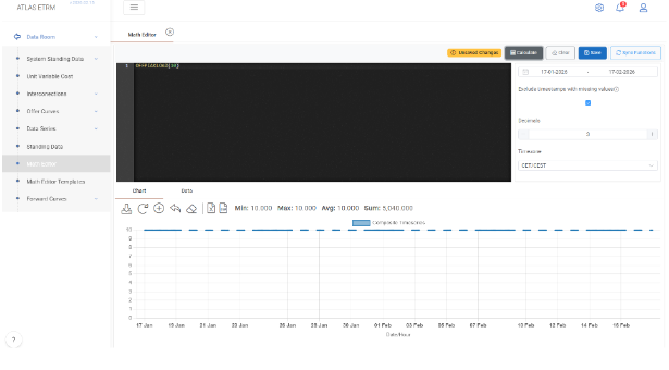
Expression 
OFFPEAKLOAD(10) 

This example generates an hourly off-peak load time series with a constant value of 10 during predefined off-peak hours. 

The OFFPEAKLOAD() function creates a synthetic hourly series that is complementary to the PEAKLOAD() definition. Specifically: 

• During Monday to Friday, between 08:00 and 20:00 (peak hours), the value is 0. 

• During all other hours (nights and weekends), the value is set to 10. 

The resulting time series has Hour granularity and automatically applies the standard peak/off-peak calendar logic. No input data series is required, as the function internally constructs the profile based on predefined weekday and time-of-day rules. 

The output is a SimpleDataNumeric series representing delivery during off-peak hours only. 

Such off-peak profiles are commonly used in electricity trading, structured contracts, tariff modelling, and settlement simulations where energy delivery occurs outside standard peak business hours. 

Example 23 – DOWNSAMPLE 

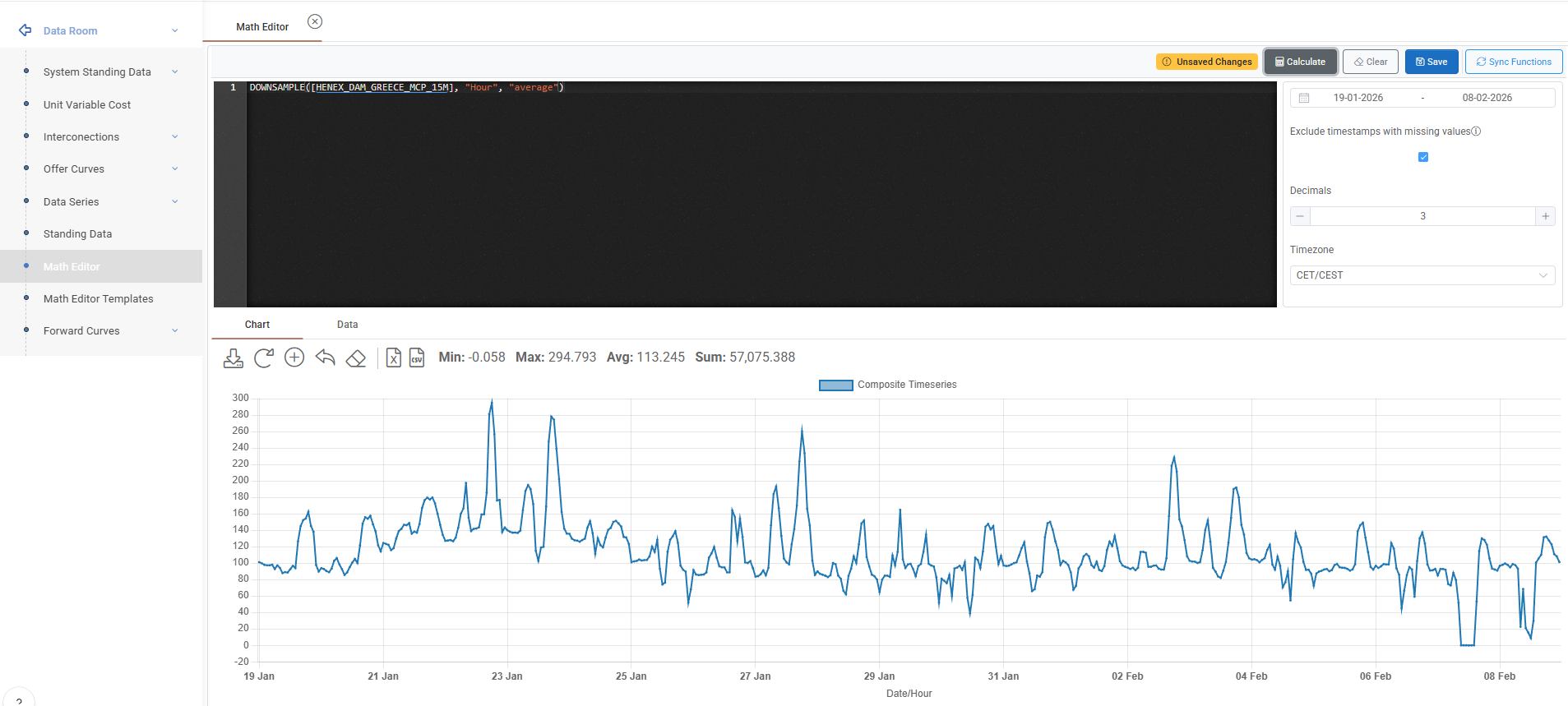
Expression 
DOWNSAMPLE([HENEX_DAM_GREECE_MCP_15M], "Hour", "average") 

This example converts the QuarterHour (15-minute) price series HENEX_DAM_GREECE_MCP_15M to Hour granularity using the average aggregation method. 

Because the original series has finer granularity (15-minute), the DOWNSAMPLE() function reduces the temporal resolution by aggregating all underlying values within each target period. In this case, the four quarter-hour price values that belong to each calendar hour are averaged, and their arithmetic mean defines the hourly value. 

The third parameter explicitly defines the aggregation method. Allowed methods include: 

• "average" (or "avg") 

• "sum" 

• "min" 

• "max" 

• "median" 

• "first" 

• "last" 

For price series, the most common aggregation method is "average", as it preserves economic interpretation when converting to coarser resolution. 

The resulting output is a SimpleDataNumeric time series with Hour granularity. Each hourly timestamp represents the aggregated value of the corresponding 15-minute observations within that hour. 

An optional fourth parameter (ignoreNulls) can be used to control null-handling behaviour. When set to true, null values are excluded from the aggregation. When false (default), the presence of null values within the aggregation window may result in a null output for that period. 

Downsampling is commonly used for reporting alignment, settlement preparation, portfolio aggregation, and analytical processes where datasets must be standardized to a coarser temporal resolution.