3.8 Forward Curves
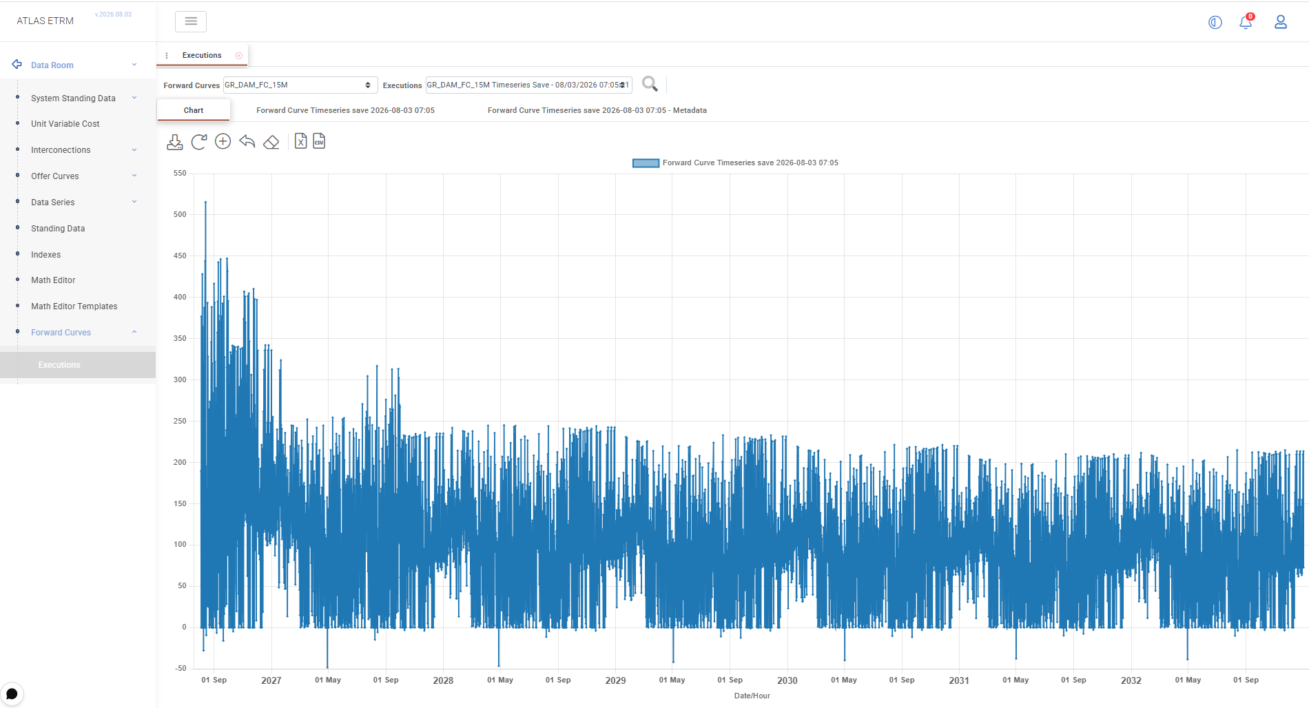
Overview
Forward curves show how market prices are expected to develop across future delivery periods. They provide a consistent price outlook that can be used for portfolio valuation, pricing and risk analysis.
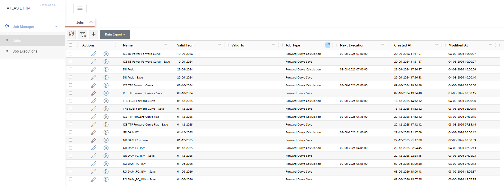
The curves are calculated and saved automatically through scheduled jobs configured in the Job Manager. The Forward Curves page brings these results together, allowing users to view each curve, inspect its underlying values and review the market data used in its calculation.
Previous executions are also retained, making it possible to compare the latest curve with earlier market expectations.
How Forward Curves Are Generated
The calculation uses available prices for traded forward and futures products together with historical prices for the relevant spot index.
Since market products may cover overlapping delivery periods, a cascading process is applied to reconcile their prices according to the non-arbitrage principle. This initially produces a flat curve that preserves the average prices represented by the available market products.
Historical spot prices can then be used to profile the flat curve at a finer granularity. This introduces the characteristic seasonal patterns of the relevant market while preserving the average prices established during the cascading process. Base-load and peak-load prices are also considered in the calculation where available.
The resulting curve may therefore be retained as a flat curve or generated with seasonality, depending on the job configuration.
The Job Manager controls the calculation schedule and the required inputs. Once the calculation and saving jobs have been configured, new results are generated and stored automatically for use across ATLAS ETRM.
Working with Forward Curves
The Forward Curves page provides access to both the latest and historical results of each configured curve. Users first select the curve they want to examine and then choose one of its saved executions. The Forward Curves field lists the available curves, while the Executions field presents the saved results by execution date and time, allowing users to review how the curve and its underlying market data have changed between calculations.
The selected execution includes three views:
Chart displays the calculated curve across its delivery horizon.
Timeseries presents the calculated price for each interval.
Metadata shows the market products and prices used to construct the curve.
The displayed data can also be exported for further analysis.
Forward Curve Metadata
The Metadata view provides details of the products used during the cascading process. For each product, it displays its type, original delivery period and market price.
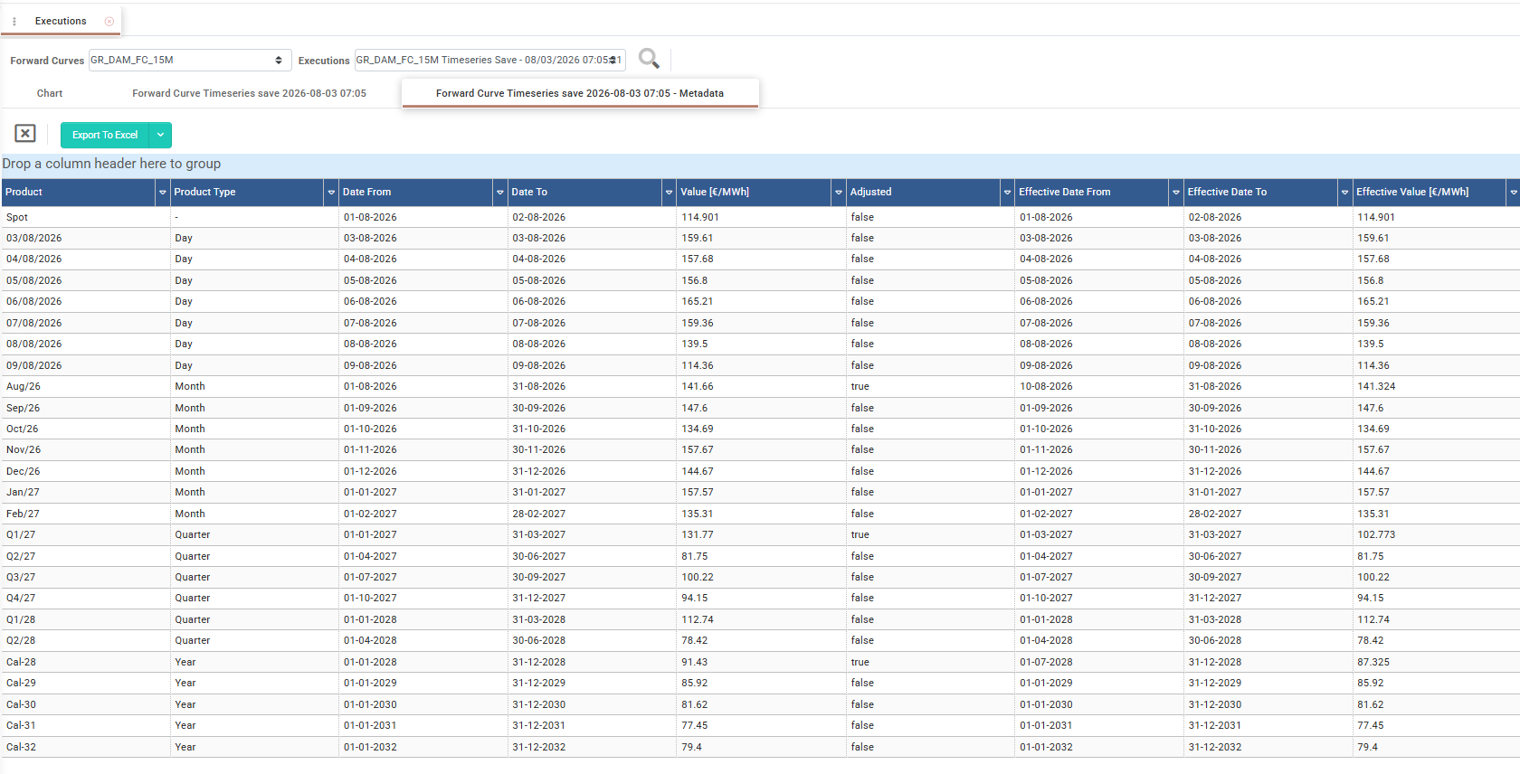
Where a product has been adjusted during cascading, the view also displays the effective delivery period and value used in the final calculation. This makes it possible to trace how the available market products contributed to the resulting curve.
Appendix - Field Details
Field / Element | Description |
|---|---|
Forward Curves | Forward curve available for selection. |
Executions | Saved results for the selected forward curve, identified by execution date and time. |
Chart | Visual representation of the calculated prices across the curve’s delivery horizon. |
Timeseries | Calculated price values for the individual intervals of the curve. |
Metadata | Market products, prices and adjustments used to construct the curve. |
Product | Name of the spot, forward or futures product used in the calculation. |
Product Type | Delivery-period classification of the product, such as Day, Month, Quarter or Year. |
Date From | Start of the product’s original delivery period. |
Date To | End of the product’s original delivery period. |
Value [€/MWh] | Original market price of the product. |
Adjusted | Indicates whether the product was adjusted during the cascading process. |
Effective Date From | Start of the delivery period represented by the product after adjustment. |
Effective Date To | End of the delivery period represented by the product after adjustment. |
Effective Value [€/MWh] | Product price resulting from the cascading adjustment and used for the effective delivery period. |
Was this helpful?