Overview
The Forward Curve Calculation job builds forward price curves from the latest prices of traded forward and futures products and the historical prices of the relevant spot index. It reconciles overlapping products through a cascading process and, where required, applies the seasonal pattern of the spot market to produce a curve at a finer granularity. The results are saved and made available in the Forward Curves page of the Data Room. The calculation method is described in 3.8 Forward Curves.
Traded products overlap in time: a year contains four quarters and a quarter contains three months. The job makes these prices consistent with each other and then breaks the curve down to the granularity of the spot series, for example hourly or 15-minute, using the shape of historical spot prices. Scheduling the job after the latest settlement prices have been loaded keeps the curves current for valuation, risk and pricing.
Input Configuration
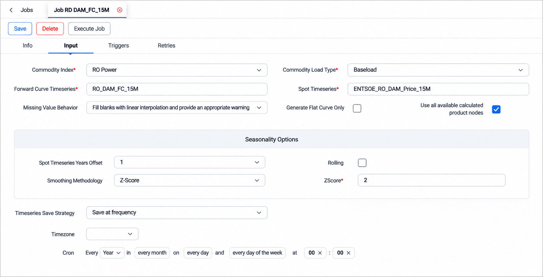
Users select the commodity index and load type whose products are used in the calculation, the timeseries in which the forward curve is stored and the spot timeseries used for profiling. They can also choose how missing values are handled, whether the curve should remain flat, and which product nodes should be included.
The Missing Value Behavior decides what happens when input prices are incomplete. Stopping the process is the safer choice when the curve feeds valuations, while interpolation keeps the curve available when occasional gaps are expected and records a warning in the execution log. Generate Flat Curve Only keeps each product at its own price without seasonal shape, which is useful for markets without a reliable spot history.
When seasonality is applied, the Seasonality Options define how many years of spot history are used and how outliers are smoothed. With Rolling selected, the history window moves forward with each execution, so the profile always reflects the most recent years. Z-Score smoothing removes extreme hours, such as price spikes, so that they do not distort the shape of the curve. The Timeseries Save Strategy determines whether the results are kept for every execution, saved at a defined frequency, or not saved. With Save at frequency, a separate schedule defines when results are stored, for example once per day.
Appendix – Field Details
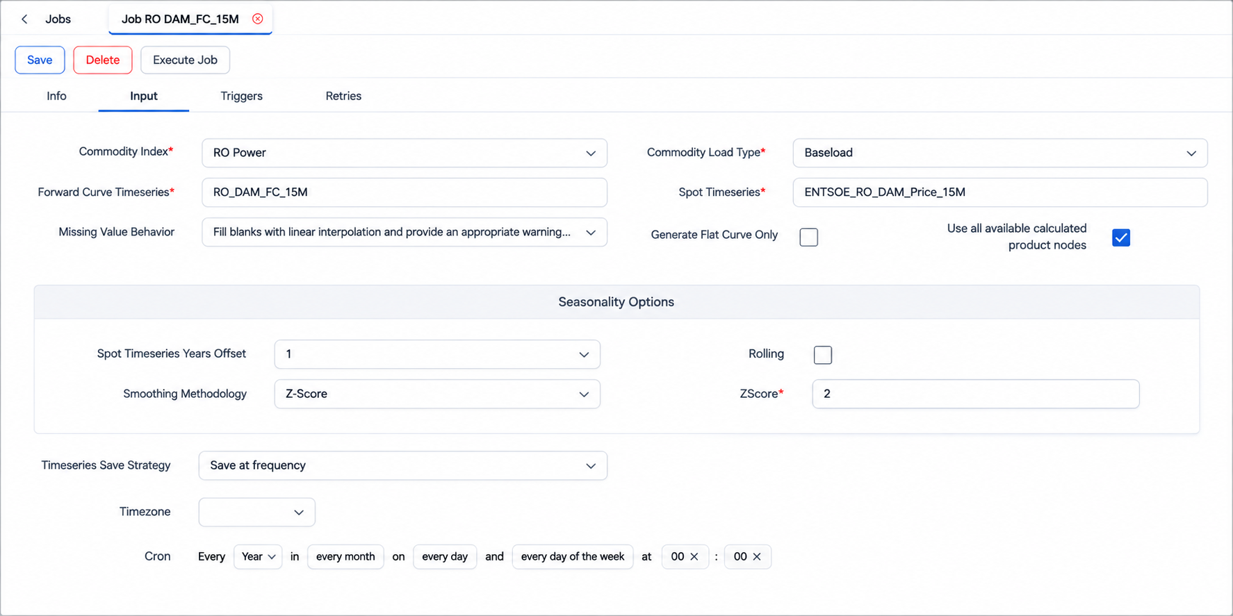
Field / Element | Required | Description |
|---|---|---|
Commodity Index | Yes | Index whose traded products are used to build the curve. |
Commodity Load Type | Yes | Load type of the commodity products used, for example Baseload. |
Forward Curve Timeseries | Yes | Timeseries in which the calculated curve is stored. |
Spot Timeseries | Yes | Historical spot price timeseries used to profile the curve. |
Missing Value Behavior | No | Stop process and create an appropriate error/fail message, or fill blanks with linear interpolation and provide an appropriate warning message. |
Generate Flat Curve Only | No | When selected, the curve is kept flat and the Seasonality Options are hidden. |
Use all available calculated product nodes | No | When selected, all available product nodes are used in the calculation. |
Only use these nodes | Yes | Product nodes included in the calculation, such as D+0, W+1, M+2, Q+1 or Y+1. |
Spot Timeseries Years Offset | No | Number of years of spot history used for seasonality, from 1 to 10. |
Rolling | No | When selected, the spot history window rolls with each execution. |
Smoothing Methodology | No | Method used to smooth outliers in the spot history: None or Z-Score. |
ZScore | Conditional | Threshold applied by the Z-Score smoothing. |
Timeseries Save Strategy | No | Do not Save, Save at frequency or Save all executions. |
Timezone | Conditional | Timezone of the saving schedule. Shown when Save at frequency is selected. |
Cron | Conditional | Saving schedule. Shown when Save at frequency is selected. |